tags:
- data-structure
- python
- algorithms
Big O Categories Review
| Big-O | Name | Description |
|---|---|---|
| O(1) | constant | Best The algorithm always takes the same amount of time, regardless of how much data there is. Example: Looking up an item in a list by index |
| O(log n) | logarithmic | Great Algorithms that remove a percentage of the total steps with each iteration. Very fast, even with large amounts of data. Example: Binary search |
| O(n) | linear | Good 100 items, 100 units of work. 200 items, 200 units of work. This is usually the case for a single, non-nested loop. Example: unsorted array search. |
| O(n log n) | linearithmic | Okay This is slightly worse than linear, but not too bad. Example: mergesort and other "fast" sorting algorithms. |
| O(n^2) | quadratic | Slow The amount of work is the square of the input size. 10 inputs, 100 units of work. 100 Inputs, 10,000 units of work. Example: A nested for loop to find all the ordered pairs in a list. |
| O(n^3) | cubic | Slower If you have 100 items, this does 100^3 = 1,000,000 units of work. Example: A triple nested for loop to find all the ordered triples in a list. |
| O(2^n) | exponential | Horrible We want to avoid this kind of algorithm at all costs. Adding one to the input doubles the amount of steps. Example: Brute-force guessing results of a sequence of n coin flips. |
| O(n!) | factorial | Even More Horrible The algorithm becomes so slow so fast, that is practically unusable. Example: Generating all the permutations of a list |
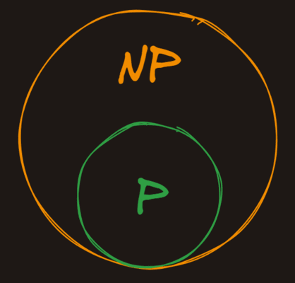
P vs NP
NP (which stands for nondeterministic polynomial time is the set of problems whose solutions can be verified in polynomial time, but not necessarily solved in polynomial time.
P is in NP
Because all problems that can be solved in polynomial time can also be verified in polynomial time, all the problems in P are also in NP.
The Oracle
A good way of thinking about problems in NP is to imagine that we have a magic oracle that gives us potential solutions to problems. Here would be our process for finding if a problem is in NP:
- Present the problem to the magic oracle
- The magic oracle gives us a potential solution
- We verify in polynomial time that the solution is correct
If we can do the verification in polynomial time, the problem is in NP, otherwise, it isn't.
Stack
- It is LIFO(Last In first out) type data structure. It is kind of list but with limitations
- All supported operations are
O(1)by themselves. However, some tasks, like getting to an item at the bottom of the stack have a higher time complexity because they require multiplepopoperations. - Stack operations are limited: no searching, no sorting, no random access
- Stacks, like all abstract data types, can store items of any type. What makes it a stack is the behavior of the operations, not the type of data it stores.
- Stacks are often used in the real world for:
- Function call management
- Undo/redo functionality
- Expression evaluation
- Browser history
Supported Operations
| Operation | Big O | Description |
|---|---|---|
| push | O(1) | Add an item to the top of the stack |
| pop | O(1) | Remove and return the top item from the stack |
| peek | O(1) | Return the top item from the stack without modifying the stack |
| size | O(1) | Return the number of items in the stack |
Code
class Stack:
    def __init__(self):
        self.items = []

    def push(self, arrow):
        self.items.append(arrow)

    def size(self):
        return len(self.items)

    def peek(self):
        if len(self.items) == 0:
            return None
        return self.items[-1]

    def pop(self):
        if len(self.items) == 0:
            return None
        item = self.items[-1]
        del self.items[-1]
        return item
[[Stacks]]
Queue
- A queue is a data structure that stores ordered item. It's like a list, but again, like a stack, its design is more restrictive. A queue only allows items to be added to the tail of the queue and removed from the head of the queue.
- It is a FIFO - first in first out data structure.
Operations
| Operation | Big O | Description |
|---|---|---|
| push / enqueue | O(1) | Add an item to the back of the queue |
| pop / dequeue | O(1) | Remove and return the front item from the queue |
| peek | O(1) | Return the front item from the queue without modifying the queue |
| size | O(1) | Return the number of items in the queue |
Code
class Queue:
    def __init__(self):
        self.items = []

    def push(self, item):
        self.items.insert(0, item)

    def pop(self):
        if len(self.items) == 0:
            return None
        temp = self.items[-1]
        del self.items[-1]
        return temp

    def peek(self):
        if len(self.items) == 0:
            return None
        return self.items[-1]

    def size(self):
        return len(self.items)

    def search_and_remove(self, item):
        if item not in self.items:
            return None
        self.items.remove(item)
        return item

    def __repr__(self):
        return f"[{', '.join(self.items)}]"
Linked List
- A linked list is a linear data structure where elements are not stored next to each other in memory. The elements in a linked list are linked using references to each other.
- The problem with our array (normal Python list) implementation of a queue was that it had
O(n)push operations. - The linked list implementation of a queue has
O(1)push operations. - . Linked lists are usually a worse choice than standard arrays because:
- They are less performant due to more memory overhead
- They are more complex to work with, debug, and reason about
- They have no random access (indexing to a specific element)
- Linked lists are a better choice than arrays in very specific circumstances because they have
O(1)insertions and deletions at both ends of the list.
Operations
| Operation | Big O | Description |
|---|---|---|
| push / insert | O(1) | Add an item to front or back of the linked list |
| pop / delete | O(1) | Remove and return the item from front or back of the linked list |
| peek | O(1) | For the item in the start or end |
| size | O(n) | Need to iterate through the whole linked list |
Code (Queue using Linked List)
class Node:
    def __init__(self, val):
        self.val = val
        self.next = None

    def set_next(self, val):
        self.next = val

    def __repr__(self):
        return self.val

class LLQueue:
    def __init__(self):
        self.tail = None
        self.head = None

    def add_to_tail(self, node):
        if self.tail is None:
            self.tail = node
            self.head = node
            return
        self.tail.next = node
        self.tail = node

    def remove_from_head(self):
        if self.head is None:
            return None
        node = self.head
        self.head = node.next
        if self.head is None:
            self.tail = None
        return node

    def __iter__(self):
        node = self.head
        while node is not None:
            yield node
            node = node.next

    def __repr__(self):
        nodes = []
        for node in self:
            nodes.append(node.val)
        return " <- ".join(nodes)
Trees
- Trees are a widely used data structure that simulate a hierarchical... well... tree structure. That said, they're typically drawn upside down - the "root" node is at the top, and the "leaves" are at the bottom.
- Trees are kind of like linked lists in the sense that the root node simply holds references to its child nodes, which in turn hold references to their children. The difference between a Linked List and a Tree is that a tree's nodes can have multiple children instead of just one.
- A generic tree structure has the following rules:
- Each node has a value and a list of "children"
- Children can only have a single "parent"
Binary Trees
- Trees aren't particularly useful data structures unless they're ordered in some way. One of the most common types of ordered tree is a Binary Search Tree or
BST. In addition to the properties we've already talked about, aBSThas some additional constraints:- Instead of an unbounded list of children, each node has at most 2 children
- The left child's value must be less than its parent's value
- The right child's value must be greater than its parent's value
- No two nodes in the
BSTcan have the same value
- By ordering the tree this way, we'll be able to add, remove, find, and update nodes much more quickly.
Operations
| Operation | Big O | Description |
|---|---|---|
| insert | O(log(n)) | inserting element into binary tree, t only requires one comparison for each level of the tree, making it O(log(n)) (at least in a balanced tree) |
| delete | O(log(n)) | delete method is O(log(n)) because, just like most B-tree operations, we don't have to search the entire tree. We only have to search one path from the root to the leaf node we want to delete.<br>The depth of the tree on average is equal to log base 2 of the number of nodes in the tree. |
Preorder Traversal
- It's called "preorder" because the current node is visited before its children. This tree: ![[Pasted image 20241130142211.png]]
- This would be traversed in this order:
4,2,1,7,6 - Sometimes it's useful (albeit a bit slow) to iterate over all the nodes in the tree.
Postorder Traversal
- It's called "postorder" because the current node is visited after its children. The following tree: ![[Pasted image 20241130142211.png]]
- This would be traversed in this order:
1,2,6,7,4
Inorder Traversal
-
An "inorder" traversal is the most intuitive way to visit all the nodes in a tree. It's called "inorder" because the current node is visited between its children. It results in an ordered list of the nodes in the tree. The following tree:
![[Pasted image 20241130142211.png]]
-
This would be traversed in this order:
1,2,4,6,7
Code
class BSTNode:
    def __init__(self, val= None):
        self.val = val
        self.left = None
        self.right = None

    '''
        1. Check if the current value is same as the value needs to be inserted, return immediately as theres should be no duplicates
        2. Check if node don't have value then set value as given value and return
        3. if value is less than current node's value and
            a. if the left node is empty then create a new left child node with the given value and return
            b. otherwise recursively call the insert method in the left child with the val and return
        4. now val should be greater than current node's value
            a. if the right node is empty then create a new right child node with the given value and return
            b. otherwise recursively call the insert method in the right child with the val
    '''
    def insert(self, val):
        if self.val == val:
            return
        if self.val is None:
            self.val = val
            return
        if val < self.val:
            if self.left is None:
                self.left = BSTNode(val)
                return
            self.left.insert(val)
            return
        if self.right is None:
            self.right = BSTNode(val)
            return
        self.right.insert(val)

    def get_min(self):
        node = self
        while node.left is not None:
            node = node.left
        return node.val

    def get_max(self):
        node = self
        while node.right is not None:
            node = node.right
        return node.val

    '''
        1. Check if the current node's value (self.val) is None. If it is, return None.
            This represents an empty tree or a leaf node where deletion has already occurred.
        2. If the value to delete (val) is less than the current node's value:
            Check if there's a left child (self.left). If it exists, recursively call the delete method on the left child with the value to delete and set the left child to the return value of the recursive call.
            Regardless of whether the left child exists or not, return the current node.
        3. Do the same (but mirrored) for the right child (self.right).
        4. If the value to delete is equal to the current node's value, we have found the node we want to delete:
            a. If there is no right child, return the left child. This effectively deletes the current node by bypassing it.
            b. If there is no left child, return the right child. This effectively deletes the current node by bypassing it.
            c. If there are both left and right children, find the minimum larger node (min_right_node) by traversing down the left side of the right subtree. This is the node with the smallest value that is still larger than self.val.
            Replace self.val with min_right_node.val.
            d. Delete min_right_node.val from the right subtree and set the right child to the return value of the recursive call.
            e. Return the current node.
    '''
    def delete(self, val):
        if self.val is None:
            return None

        if self.val > val:
            if self.left is not None:
                self.left = self.left.delete(val)
            return self


        if self.val < val:
            if self.right is not None:
                self.right = self.right.delete(val)
            return self

        if self.right is None:
            return self.left

        if self.left is None:
            return self.right

        min_right_node = self.right
        while min_right_node.left is not None:
            min_right_node = min_right_node.left
        self.val = min_right_node.val
        self.right = self.right.delete(min_right_node.val)
        return self

    '''
        1. Visit the value of the current node by appending its value to the visited array
        2. Recursively traverse the left subtree
        3. Recursively traverse the right subtree
        4. Return the array of visited nodes
        for the root node call will be tree.preorder([])
    '''
    def preorder(self, visited):
        visited.append(self.val)
        if self.left:
            self.left.preorder(visited)
        if self.right:
            self.right.preorder(visited)
        return visited

    '''
        1. Recursively traverse the left subtree
        2. Recursively traverse the right subtree
        3. Visit the value of the current node by appending its value to the visited array
        4. Return the array of visited nodes
    '''
    def postorder(self, visited):
        if self.left:
            self.left.postorder(visited)
        if self.right:
            self.right.postorder(visited)
        visited.append(self.val)
        return visited

    '''
        1. Recursively traverse the left subtree
        2. Visit the value of the current node by appending its value to the visited array
        3. Recursively traverse the right subtree
        4. Return the array of visited nodes
    '''
    def inorder(self, visited):
        if self.left:
            self.left.inorder(visited)
        visited.append(self.val)
        if self.right:
            self.right.inorder(visited)
        return visited

    '''
        To check if the node is exist in the tree or not
        Return True if found the node else False
    '''
    def exists(self, val):
        if self.val == val:
            return True
        if self.left:
            return self.left.exists(val)
        if self.right:
            return self.right.exists(val)
        return False

    '''
        Returns all elements with the specified range from the tree in sorted order
        This uses inorder traversal to traverse tree
    '''
    def search_range(self, lower_bound, upper_bound):
        result = []
        if self.val is None:
            return result
        if self.left and self.val > lower_bound:
            result.extend(self.left.search_range(lower_bound, upper_bound))
        if lower_bound <= self.val <= upper_bound:
            result.append(self.val)
        if self.right and self.val < upper_bound:
            result.extend(self.right.search_range(lower_bound, upper_bound))
        return result


    '''
        Returns depth of the tree
        1. If the node's value is None, return 0.
        2. Recursively calculate the height of the left subtree.
        3. Recursively calculate the height of the right subtree.
        4. Return the maximum of the left and right subtree heights plus 1.
    '''
    def height(self):
        if self.val is None:
            return 0
        left_depth = 0
        if self.left:
            left_depth = self.left.height()
        right_depth = 0
        if self.right:
            right_depth = self.right.height()
        return max(left_depth, right_depth) + 1
Red Black Tree
- BST's have a problem. While it's true that on average a
BSThasO(log(n))lookups, deletions, and insertions, that fundamental benefit can break down quickly if most of data is sorted or completely sorted than the depth of the tree will be very huge than the width and which increase the complexity. - A red-black tree is a kind of binary search tree that solves the "balancing" problem. It ensure that as nodes are inserted and deleted, the tree remains relatively balanced.
- Each node in an RB Tree stores an extra bit, called the "color": either red or black. The "color" ensures that the tree remains approximately balanced during insertions and deletions. When the tree is modified, the new tree is rearranged and repainted to restore the coloring properties that constrain how unbalanced the tree can become in the worst case.
Rules
- In addition to all the rules of a Binary Search Tree, a red-black tree must follow some additional ones:
- Each node is either red or black
- The root is black. This rule is sometimes omitted. Since the root can always be changed from red to black, but not necessarily vice versa, this rule has little effect on analysis.
- All
Nilleaf nodes are black. - If a node is red, then both its children are black.
- All paths from a single node go through the same number of black nodes to reach any of its descendant
NILnodes.
Rotations
- Rotations are what actually keeps red-black tree balanced.
- This operation is the O(1).
- A properly-ordered tree pre-rotation remains a properly-ordered tree post-rotation
- When rotating left:
- The "pivot" node's initial parent becomes its left child
- The "pivot" node's old left child becomes its initial parent's new right child ![[Pasted image 20241130215023.png]]
Code
class RBNode:
    def init(self, val):
        self.red = False
        self.parent = None
        self.val = val
        self.left = None
        self.right = None


class RBTree:
    def init(self):
        self.nil = RBNode(None)
        self.nil.red = None
        self.nil.left = None
        self.nil.right = None
        self.root = self.nil

    def insert(self, val):
        new_node = RBNode(val)
        new_node.left = self.nil
        new_node.right = self.nil
        new_node.red = True

        parent = None
        current = self.root
        while current != self.nil:
            parent = current
            if val < current.val:
                current = current.left
            elif current.val < val:
                current = current.right
            else:
                return

        new_node.parent = parent
        if parent is None:
            self.root = new_node
        if val < parent.val:
            parent.left = new_node
        else:
            parent.right = new_node
        self.fix_insert(new_node)

    def fix_insert(self, new_node):
        while new_node.parent is not None and new_node.parent.red:
            parent = new_node.parent
            grandparent = parent.parent
            if parent == grandparent.right:
                uncle = grandparent.left
                if uncle.red:
                    uncle.red = False
                    parent.red = False
                    grandparent.red = True
                    new_node = grandparent
                else:
                    if new_node == parent.left:
                        new_node = parent
                        self.rotate_right(new_node)
                    parent.red = False
                    grandparent.red = True
                    self.rotate_left(grandparent)
            else:
                uncle = grandparent.right
                if uncle.red:
                    uncle.red = False
                    parent.red = False
                    grandparent.red = True
                    new_node = grandparent
                else:
                    if new_node == parent.right:
                        new_node = parent
                        self.rotate_left(new_node)
                    parent.red = False
                    grandparent.red = True
                    self.rotate_right(grandparent)
        self.root.red = False

    def rotate_left(self, pivot_parent):
        if pivot_parent == self.nil or pivot_parent.right == self.nil:
            return
        pivot = pivot_parent.right
        pivot_parent.right = pivot.left
        if pivot.left != self.nil:
            pivot.left.parent = pivot_parent
        pivot.parent = pivot_parent.parent
        if pivot_parent.parent is None:
            self.root = pivot
        elif pivot_parent.parent.val < pivot_parent.val:
            pivot_parent.parent.right = pivot
        else:
            pivot_parent.parent.left = pivot
        pivot.left = pivot_parent
        pivot_parent.parent = pivot

    def rotate_right(self, pivot_parent):
        if pivot_parent == self.nil or pivot_parent.left == self.nil:
            return
        pivot = pivot_parent.left
        pivot_parent.left = pivot.right
        if pivot.right != self.nil:
            pivot.right.parent = pivot_parent
        pivot.parent = pivot_parent.parent
        if pivot_parent.parent is None:
            self.root = pivot
        elif pivot_parent.val < pivot_parent.parent.val:
            pivot_parent.parent.left = pivot
        else:
            pivot_parent.parent.right = pivot
        pivot.right = pivot_parent
        pivot_parent.parent = pivot
HashMap
- A hash map or "hash table" is a data structure that maps keys to values:
"bob" -> "ross"
"pablo" -> "picasso"
"leonardo" -> "davinci"
- The lookup, insertion, and deletion operations of a hashmap have an average computational cost of
O(1). Python's dictionary is an example of a hashmap. - In Python, that means dictionaries. In Go, it means maps. In JavaScript, it means object literals. The point is, if you need an in-memory key-value store, hashmaps are awesome, and every language tends to have a built-in implementation.
Under the hood
- The hashmap are built on top of the Array's. They use a hash function to convert a "hashable" key into an index in the array. From a high-level, all that matters to us is that the hash function:
- Takes a key and returns an integer.
- Always returns the same integer for the same key.
- Always returns a valid index in the array (e.g. not negative, and not greater than the array size)
- Ideally the hash function hashes each key to a unique index, but most hash table designs employ an imperfect hash function, which might cause hash collisions where the hash function generates the same index for more than one key.
Properties of a good Hash map
- Fast Lookups: Hash maps have an average time complexity of
O(1)for lookups, insertions, and deletions. - Unordered: Hash maps (typically) do not guarantee any particular order of keys.
- No Ranging: While hash maps are great for lookups, they don't provide the ability to look into a range of keys (e.g. the largest ten keys). That's one reason production databases like Postgres use binary trees for indexing.
- Collision Resistant: Hash maps are built on top of arrays and use a hash function to convert a key into an index. Production-ready implementations (like Python dictionaries) handle hash collisions and make them a non-issue in practice.
- Hashable Keys: Keys must be hashable. This means they must be immutable and have a consistent hash value. For example, in Python, a tuple can be a key, but a list cannot.
- Efficient Resizing: When a hashmap's capacity is exceeded, it dynamically resizes (usually by doubling in size) and rehashes the elements. A good hash map manages this resizing efficiently, minimizing performance hits.
- Uniform Distribution: A good hash function ensures keys are distributed evenly across the hashmap's underlying array, minimizing the number of collisions and optimizing lookup speed.
Handling collisions
- Linear Probing: It works by finding next available slot after the collision index and placing the data there. When collision happens we start finding next available index by going sequentially from the collision index.
Code of basic Hash map
from functools import reduce

class HashMap:
    def __init__(self, size):
        self.hashmap = [None for i in range(size)]

    def get(self, key):
        idx = self.key_to_index(key)
        if self.hashmap[idx] is None:
            raise KeyError("key not found")
        return self.hashmap[idx][1]

    def key_to_index(self, key):
        sum = 0
        for c in key:
            sum += ord(c)
        return sum % len(self.hashmap)

    '''
        Implemented resize mechanism if hashmap seems to be full
    '''
    def resize(self):
        if len(self.hashmap) == 0:
            self.hashmap = [None]
            return
        current_filled = self.current_load()
        if (current_filled * 100) < 5:
            return
        key_values = [ele for ele in self.hashmap if ele is not None]
        self.hashmap = [None for i in range(len(self.hashmap) * 10)]
        for key, val in key_values:
            self.insert(key, val)

    '''
        Implemented linear probing mechanism to avoid collisions and also resize when needed
    '''
    def insert(self, key, value):
        self.resize()
        idx = self.key_to_index(key)
        while self.hashmap[idx] is not None:
            idx = (idx + 1) % len(self.hashmap)
        self.hashmap[idx] = (key, value)

    def get(self, key):
        idx = self.key_to_index(key)
        org_idx = idx
        iter = True
        while (org_idx == idx and iter) or self.hashmap[idx]:
            if self.hashmap[idx][0] == key:
                return self.hashmap[idx][1]
            idx = (idx+1) % len(self.hashmap)
        raise Exception("sorry, key not found")

    def __repr__(self):
        final = ""
        for i, v in enumerate(self.hashmap):
            if v != None:
                final += f" - {str(v)}\n"
        return final
Tries
- A Trie is a specialized tree-like data structure that organizes and stores words in an efficient manner. Each node in a Trie represents a single character of a word, allowing for efficient addition, retrieval, and deletion of words.
- In simpler terms, a Trie is an advanced information retrieval data structure. It outperforms more conventional data structures like Hashmaps and Trees in terms of the time complexity for various operations, making it particularly useful for tasks involving large sets of strings or words.
- A trie is also often referred to as a "prefix tree" because it can be used to efficiently find all of the words that start with a given prefix.
- A trie is easily implemented as a nested tree of dictionaries where each key is a character that maps to the next character in a word. For example, the words:
- hello
- help
- hi
- Would be represented as:
{
	"h": {
		"e": {
			"l": {
				"l": {
					"o": {
						"*": True
					}
				},
				"p": {
					"*": True
				}
			}
		},
		"i": {
			"*": True
		}
	}
}
The * character is used to indicate the end of a word.
Prefix Matching
- Tries tend to be most useful for prefix matching. For example, if you wanted to find all the words in a dictionary that start with a given prefix, a trie works great! Autocomplete, keyword search, and spellcheck are all good examples of where a trie can be useful.
- Remember, a hash table is only good for exact matches, whereas a trie allows you to look up all of the words that match a given prefix.
class Trie:
    def search_level(self, cur, cur_prefix, words):
        if self.end_symbol in cur:
            words.append(cur_prefix)
        for letter in sorted(cur.keys()):
            if letter != self.end_symbol:
                self.search_level(cur[letter], cur_prefix + letter, words)
        return words

    def words_with_prefix(self, prefix):
        words = []
        current = self.root
        for letter in prefix:
            if letter not in current:
                return []
            current = current[letter]
        return self.search_level(current, prefix, words)
Find Matches
- Tries are super efficient when it comes to finding substrings in a large document of text.
class Trie:
    def find_matches(self, document):
        matches = set()
        for i in range(len(document)):
            level = self.root
            for j in range(i, len(document)):
                ch = document[j]
                if ch not in level:
                    break
                level = level[ch]
                if self.end_symbol in level:
                    matches.add(document[i : j + 1])
        return matches
Longest Common Prefix
class Trie:
    def longest_common_prefix(self):
        curr = self.root
        prefix = ""
        while True:
            if self.end_symbol in curr:
                break
            dict_keys = list(curr.keys())
            if len(dict_keys) == 1:
                prefix += dict_keys[0]
                curr = curr[dict_keys[0]]
            else:
                break
        return prefix
Code
class Tries:
    def __init__(self):
        self.root = {}
        self.end_symbol = "*"

    def add(self, word):
        curr = self.root
        for letter in word:
            if letter not in curr:
                curr[letter] = {}
            curr = curr[letter]
        curr[self.end_symbol] = True

	def exists(self, word):
        curr = self.root
        for letter in word:
            if letter not in curr:
                return False
            curr = curr[letter]
        if self.end_symbol in curr:
            return True
        return False
Dynamic Programming
[[Dynamic Programming]]